Last updated on July 19, 2015
This post is not about Gladwellian pabulum. Rather, it is about the econometric problem posed by outliers, whose presence of extreme-valued observations in a data set whose presence might cause problems of estimation and inference, and which a few colleagues have asked for a ‘Metrics Monday post on a few weeks ago.
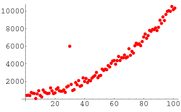
Outliers cause estimation problems because they bias point estimates. They cause inference problems because they cause standard errors to be too large, thereby making it more likely that one will fail to reject a false null, i.e., a type II error. For example, if you collect data on a random sample of the population, the bulk of the people in your data might be between 18 and 80 years old, but you might also have someone in there who is 110 years old–that person is an outlier. Or the bulk of your sample might be making between $30,000 and $300,000 a year, but you might also have someone in there who makes $200,000,000 a year–that person is also an outlier.
When I was asked for a post about outliers, I had no particular insight on the topic, so I turned to the Econometric Volume of Sacred Law, i.e., the late Peter Kennedy’s Guide to Econometrics, to see how I should tackle the topic.
Kennedy makes an important distinction: outliers vs. leverage points. An outlier is an observation whose residual is significantly larger than that of other observations (i.e., an outlier is measured along the y-axis). A leverage point is an observation that has an exceedingly low or large value of an explanatory variable (i.e., a leverage point is measured along the x-axis).
The issue with outliers and leverage points–“influential observations,” as per Kennedy’s terminology–is that they can drive your results. Usually, the best way to detect influential observations is exploratory data analysis–plot the data and see whether there are such observations. If there are, Kennedy advises taking a look at each such observation, and try to determine whether it has a story to tell (e.g., a household may report a yield of zero because lightning fell on its plot and burned the entire crop), or whether it looks like an error (e.g., a typo in data entry, or a respondent trolling the enumerator). When an observation is influential because it looks like an error, it is reasonable to throw it out.
If you keep those influential observations (say, because they have a story to tell), Kennedy suggests five different “robust” estimators on page 347, including M-estimators, which assigns weights to each observation that are not increasing in their error (OLS weights each observation in an increasing manner as it moves away from the average because it squares each error).
What I have done in my own work has been one of a few things:
- Estimate a median regression version of my regression of interest, which estimates the median instead of the mean regression slope, the median being less sensitive to outliers than the mean. It’s what I have done, for example, in this article on whether mobile phones are associated with higher prices for farmers.
- Estimate a number of other robust specifications, e.g., M-estimators, MM-estimators, S-estimators, and MS-estimators. My friend Vincenzo Verardi, who was a colleague of mine when I was on sabbatical at the University of Namur in 2009-2010, has done a bunch of work on outliers (see here for a Hausman-type test to detect outliers), and he has written a Stata add-on command to estimate those. We have also estimated those in our article on mobile phones when a reviewer asked to see some robustness checks.
- Adopt a rule of thumb for deletion of outliers–say, drop all observations that are more than 2, 2.5, or 3 standard deviations from the mean of each explanatory variable–and re-estimate everything. It’s what we did in our 2013 AJAE article on price risk.
Ultimately, what you should aim for is to show what happens across a number of estimators, i.e., OLS with outliers arbitrarily removed, robust M/S/MM/MS estimators, median regression, OLS with rule-of-thumb deleted observations, etc. If your core results are essentially the same in sign and significance across all specifications, then you should be good to go.
Note how a lot of the advice in applied econometrics is to estimate a bunch of different specifications of or a bunch of different estimators for the same specification, and see if your core result remains unchanged, which is perhaps the best indication that applied econometrics is a craft, more are than science, which one learns not by reading textbooks but by applying one’s working tools.
Thanks for taking the time to put this post together Marc. I think outliers are an under-discussed topic in much of economics. And they really can influence results.
I agree with your (familiar) idea of approaching possible outliers from multiple directions. Your leverage points suggestion reminds me of my adviser’s (Carl Nelson) assistance in calculating leverage and dfbeta statistics in our Mexico food price increases Food Policy paper. He suggested Rousseeuw and Zomeren (1990) and Bollen and Jackman, (1985) as good resources for understanding this issue.
From a replication perspective, I would like to put in a plug for more outlier transparency (in online appendices?), in both how they were identified and when/if they were removed from their data.