Last updated on December 18, 2016
From Wikipedia:
Simpson’s paradox, or the Yule-Simpson effect, is a paradox in probability and statistics, in which a trend appears in different groups of data but disappears or reverses when these groups are combined. … This result is often encountered in social-science and medical-science statistics, and is particularly confounding when frequency data is unduly given causal interpretations. The paradoxical elements disappear when causal relations are brought into consideration.
What does this mean, specifically? Suppose you are estimating the equation
(1) [math]y = {\alpha} + {\gamma}{D} + {\epsilon}[/math]
with observational (i.e., nonexperimental) data, and you are interested in the causal effect of [math]D[/math] on [math]y[/math]. Suppose further that after estimating equation (1), you find that [math]\hat{\gamma} < 0[/math].
The model in equation (1) is parsimonious–beyond the variable of interest [math]D[/math], it does not control for anything else. Suppose you decide to include a control variable [math]x[/math] and estimate the equation
(2) [math]y = {\alpha} +{\beta}{x }+ {\gamma}{D} + {\epsilon}[/math]
with the same observational data. Simpson’s paradox arises from the fact that it is entirely possible that [math]\hat{\gamma} > 0[/math] once you control for the additional control variable [math]x[/math].
In other words, without a research design that attempts to disentangle the presumed causal relationship flowing from [math]D[/math] to [math]y[/math] from the correlation between the two, the inclusion of specific control variables might well flip the sign of the estimated relationship between [math]y[/math] and [math]D[/math], i.e., of your estimate [math]{\beta}[/math] of [math]\frac{{\partial}{y}}{{\partial}{D}}[/math].
To see this graphically, consider the following figure, also from Wikipedia:
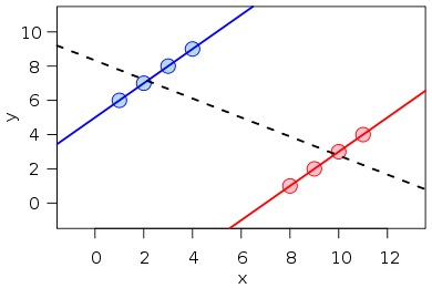
Here, just regressing [math]y[/math] on [math]x[/math] would yield a negative estimate of [math]{\beta}[/math], but controlling for the groups represented by the blue and red lines (say, with a dummy variable for blue or one for red) would flip the sign of that estimate.
Why “Determinants of …” Papers are Problematic
The foregoing illustrates why “determinants of …” or “correlates of …” papers are problematic. By “determinants of…” papers, I mean papers that lack a research design, which simply regress an outcome of interest on a number of control variables, and often use causal language to tell stories about the association between various control variables (for without a research design, that is what they are) and the outcome of interest.
Don’t get me wrong; “determinants of …” papers can be useful. For example, if you are interested in looking at who adopts some treatment [math]D[/math], a linear projection of the treatment variable on a vector of controls can help uncover some useful correlations that can help target incentives for take-up of the treatment. For example, suppose you are interested in getting people to take a multivitamin every day and you find, using a “determinants of …” analysis, that less educated people tend not to take a multivitamin every day. In that case, the analysis can help you provide stronger incentives for less educated people to take a multivitamin (say, via promotion materials targeted at them, a monetary reward for doing so, etc.) But “determinants of …” papers become problematic when a causal interpretation is given to their results, and when those results become just-so stories.
With that said, if you have to write a “determinants of …” paper at some point, the key to minimizing the problem highlighted by Simpson’s paradox is to start from the most parsimonious specification you can think of (usually, just the outcome variable regressed on one variable of interest) and show progressively less parsimonious specifications, building it up to a full-blown specification that includes all the controls you want to include. In this case, if most of your coefficients remain stable as you add in or subtract out controls, then perhaps it is the case that Simpson’s paradox is not a big deal in the context you are looking at.
Alternatively, it is sometimes the case that a good descriptive analysis will yield insights that are similar if not better than a “determinants of …” analysis, or that the latter can supplement the former to form a better descriptive picture.
When Is Simpson’s Paradox Not an Issue?
Let’s take a look at the last sentence of the definition given above, viz.
The paradoxical elements disappear when causal relations are brought into consideration.
What does this means? It simply means that once you have a research design that allows identifying the causal relationship between [math]D[/math] and [math]y[/math], Simpson’s paradox is no longer an issue.
For example, suppose you have a research design wherein you randomly assign the value of [math]D[/math] to each individual in your sample and then observe [math]y[/math]. In that case, you could collect data on a number of controls [math]x[/math] and include them in a regression of [math]y[/math] on [math]D[/math], and the sign of your estimate of [math]{\gamma}[/math] would not change–the only thing that would happen would be that the standard error around your estimate of [math]{\gamma}[/math] would shrink, and your estimate would become more precise.