Last updated on February 5, 2017

It sometimes happens that in the general regression equation
(1) [math]y_{i} = \alpha + \beta {x}_{i} + \epsilon_{i}[/math],
your outcome of interest will be a length of time, or duration. Classic examples from labor economics are the duration of individual unemployment spells, or the duration of a strike.
The problem with duration data is that they do not look like the continuous outcome variable ranging from minus to plus infinity (ideally normally distributed) found in most introductory textbooks. In the unemployment spell example, we typically know when someone loses their job, and we know when they find another one. Sometimes, however, the duration is censored; that is, we know when someone loses their job, but they remain unemployed when we record the data.
In both cases, the data look nothing like the textbook outcome variable, and so special care might be required in how we deal with a duration on the left-hand side of equation (1). Typically, this is done with duration analysis, as it is known in economics. Those are also known as survival models–a term that comes from the biostatistics, in which researchers are often interested in how long someone survives after some event of interest happens–but that is only one of the many names given to duration analysis.*
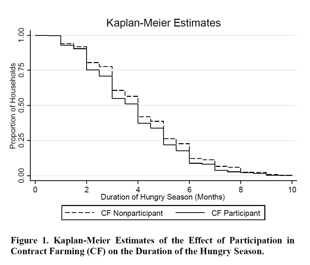
The most basic type of duration analysis is entirely nonparametric, and it is referred to as the Kaplan-Meier estimator. More than an “estimator,” it really is a graph which plots length of time on the x-axis and the proportion of the sample that remains in a given state on the y-axis. Predictably, a Kaplan-Meier plot looks like a descending staircase.
Here is an example from Bellemare and Novak (forthcoming),** in which we look at whether participating in contract farming (CF) reduces the duration of the hungry season (i.e., the length of time household members go without eating three meals a day) experienced by the households in the data.
Obviously, this fails to account for any confounding factor. For that, you need specific estimators. The two we use in Bellemare and Novak are the Cox proportional hazards model*** and the survival-time regression. The Cox proportional hazards model is such that
(2) [math]h(t)=h_{0} (t)\exp\{\beta {x}\}[/math],
where [math]x[/math] is defined as in equation 1, but where [math]h_{i}(t)[/math] denotes the “hazard” at time t, i.e., the likelihood at time t that an observation will exit the condition studied (in Bellemare and Novak, the likelihood at time t that a household will exit the hungry season), and [math]h_{0i}(t)[/math], the same hazard at baseline. (The Stata help file for the Cox proportional hazards command notes that hazard at baseline is not directly estimated, but it is possible to recover it.)
The survival-time regression, in its proportional hazards version, is such that
(3) [math]h(t)=h_{0} (t)g(x)[/math],
where [math]g(x)[/math] is a nonnegative function of the covariates (typically [math]\exp\{\beta {x}\}[/math]). Without specifying [math]h_{0} (t)[/math], equation (3) reverts to equation (2), so the Cox proportional hazards model is nested within the survival-time estimator.
A survival-time regression involves a survival function [math]S(t)[/math], which is inversely related to the hazard function, i.e., it measures the probability of survival until time t (in Bellemare and Novak, the probability of having a hungry season of length t). The catch is that you have to make a specific distributional assumption if you want to estimate a (parametric) survival-time regression. The most popular choice appears to be Weibull, and this is what we adopted in our paper.
Now, the really cool thing about using these estimators along with the usual linear regression for robustness is this: Whereas the linear regression will tell you the effect of an increase of [math]x[/math] by one unit on the duration of interest for the average observation, both the Cox proportional hazards and survival-time regressions will tell you how much more likely the average observation is to exit the condition you are studying in response to an increase of [math]x[/math] by one unit.
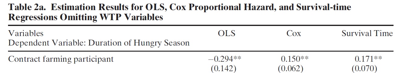
In Bellemare and Novak, combining duration analysis with linear regressions tells us that participation in contract farming is associated with a hungry season that is 0.29 months (about eight days) shorter on average (as per the OLS results above), but also that it is associated with a likelihood of exiting the hungry season at any given time that is 15 or 17.1 percent (depending on whether you look at the Cox proportional hazards or survival time results) higher for participating households than it is for nonparticipating households. Both those results answer related but very different questions.
As always, a word of caution. The estimators just discussed work really well with an experimental design or with a selection-on-observables design, but I wouldn’t want to have to use them with an obviously endogenous variable of interest. In Bellemare and Novak, we could make the case that we had selection on observables, but if we had had to deal with an instrumental variable, for example, we would have stuck to trusty old OLS specifications.
* From the Wikipedia entry on survival analysis: “This topic is called reliability theory or reliability analysis in engineering, duration analysis or duration modelling in economics, and event history analysis in sociology.”
** I must confess that one of my initial reasons for wanting to write that paper was that I had never written anything involving the use of duration data. Little did I know it was to evolve into a piece from which we learn quite a bit about the welfare impacts of contract farming on outcomes other than income.
*** One day I will write a post about how much the use of the term “model” to designate a regression equation or an estimator grinds my gears. One day.