(Update: There was a mistake in the original post. Thanks to Peter Hull, Paul Hünermund, Vincent Arel-Bundock, and Daniel Millimet, who provided enlightening comments on the original post, the proper procedure is given at the bottom, along with some ideas for implementation in Stata.)
If you have been reading this blog for a while, you are undoubtedly familiar with the usual methods used by economists to identify causal relations (e.g., randomized controlled trials, instrumental variables, difference-in-differences, etc.)
One method that you may not have heard of, or that you might only have heard of in passing, is Pearl’s (2000) front-door criterion, which Pearl discusses in a more intuitive way in The Book of Why, the popular-press book he has recently published in which he discusses his work on causality (Pearl, 2018). In fact, in The Book of Why, Pearl goes so far as to assert that the use of the front-door criterion might help end the hegemony of randomized controlled trials when it comes to identifying causal impacts!
Consider the following figure, where X denotes a treatment variable, Y denotes the outcome of interest, M denotes a mechanism through which X causes Y, and U represents unobserved confounders.
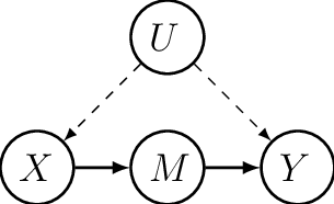
Let’s ignore M for a minute. If you have ever seen a graph like the one in the figure above–a directed acyclic graph, or DAG–that type of graph is used by causality researchers to look at the structure underlying a causal model. Here, the identification problem is illustrated by the fact that U affects both X and Y (i.e., there are arrows from U to both X and Y), and that is the reason why identifying the causal relationship flowing from X to Y is difficult, i.e., because any correlation between the two cannot be argued to be causal because of the presence of U. In such cases, an economist’s first instinct would often be to find a variable Z which is correlated with X but which is not affected by U–a setup which would allow identifying the causal effect of X on Y, and which you have probably recognized as an instrumental variable (IV) setup.
Pearl, however, came up with a clever way of identifying the causal effect of X on Y which tends to be somewhat less demanding than having to find a credible IV. Looking at the figure above, Pearl’s method involves finding a mechanism M whereby X causes Y, but which is itself not affected by unobserved confounders. (Indeed, notice that there is no arrow from U to M in the figure above.)
That is essentially the idea of the front-door criterion: To find a mechanism M whereby X causes Y but which is not itself affected by unobserved confounders. In an old post, Alex Chinco, an assistant professor of finance at the University of Illinois, explains how even in the presence of self-selection of units into treatment, if you can credibly make the case that treatment intensity is not affected by the unobserved confounders that drive both the uptake of treatment and your outcome of interest, you can identify the effect of the treatment on that outcome.
Intuitively, what the front-door criterion does is kind of like what IV does, except that it moves the variable that purges the variation in X from its correlation with U in front of X (hence the name front-door criterion), or between X and Y such that you have X -> M -> Y, instead of behind it (as in a traditional 2SLS setup) where you have Z -> X -> Y.
It took me a while to sit down to write this post, because the idea behind this series of posts is to present things that one can use in a regression context, and whatever I have read from Pearl usually presents the front-door criterion in a simple binary treatment, binary outcome, and binary mechanism example involving smoking as treatment, lung cancer as outcome, and the rate of tar accumulation in the lungs as mechanisms, in which case you can recover the treatment effect by multiplying conditional probabilities.
But applied economists usually are interested in examples that involve more than just binary variables, and it took me a while to find a discussion of how to do this in a regression context. Even the recent paper by Glynn and Kashkin (2017) comparing front and backdoor criteria does not go into the details of how to do that. Luckily, the Alex Chinco post I refer to above goes into the details of how to do that. Specifically, Chinco discusses a two-step procedure, as follows. In a discussion about how to implement this in practice on Twitter, here is what came up (though reddit user /u/unistata came up with it six months before):
- Regress M on X and a constant.
- Regress Y on M, X, and a constant.
- Multiply the coefficient on X in step 1 by the coefficient on M in step 2.
The result of step 3 is then the front-door criterion estimate of the causal effect of treatment X on outcome Y.
How would you implement this in Stata. A quick and dirty way to do it would to estimate
. sureg (m x) (y m x)
. nlcom [m]_b[x]*[y]_b[m]
As always, there is no free lunch, and in order to apply the front-door criterion, one has to make the case that M really is not affected by U the way X and Y are, which might be a difficult case to make. But if you have an application where self-selection into treatment compromises the identification of the causal effect of treatment on your outcome of interest and you can find a variable that measures the intensity of that treatment which is not driven by the same confounding factors as those affecting treatment and outcome, you might have a good case for using the front-door criterion.