Last updated on January 20, 2019
A long time ago I promised myself that I would not become one of those professors who gets too comfortable knowing what he already knows. This means that I do my best to keep up-to-date about recent developments in applied econometrics.
So my incentives in writing this series of post isn’t entirely selfless: Because good (?) writing is clear thinking made visible, doing so helps me better understand econometrics and keep up with recent developments in applied econometrics.
By “applied econometrics,” I mean applied econometrics almost exclusively of the causal-inference-with-observational-data variety. I haven’t really thought about time-series econometrics since the last time I took a doctoral-level class on the subject in 2000, but that’s mostly because I don’t foresee doing anything involving those methods in the future.
One thing that I don’t necessarily foresee using but that I really don’t want to ignore, however, is machine learning (ML), especially since ML methods are now being combined with causal inference techniques. So having been nudged by Dave Giles’ post on the topic earlier this week, I figured 2019 would be a good time–my only teaching this spring is our department’s second-year paper seminar, and I’m on sabbatical in the fall, so it really is now or never.
I’m not a theorem prover, so I really needed a gentle, intuitive introduction to the topic. Luckily, my friend and office neighbor Steve Miller also happens to teach our PhD program’s ML class and to do some work in this area (see his forthcoming Economics Letters article on FGLS using ML, for instance), and he recommended just what I needed: Introduction to Statistical Learning, by James et al. (2013).
The cool thing about James et al. is that it also provides an introduction to R for newbies. Being such a neophyte, going through this book will provide a double learning dividend for me. Even better is the fact that the book is available for free on the companion website (which features R code, data sets, etc.) here.
I’m only in chapter 2, but I have already learned some new things. Most of those things have to do with new terminology (e.g., supervised learning wherein you have a dependent variable, vs. unsupervised learning, wherein there is no such thing as a dependent variable), but here is one thing that was new to me: The idea that there is a tradeoff between flexibility and interpretability.
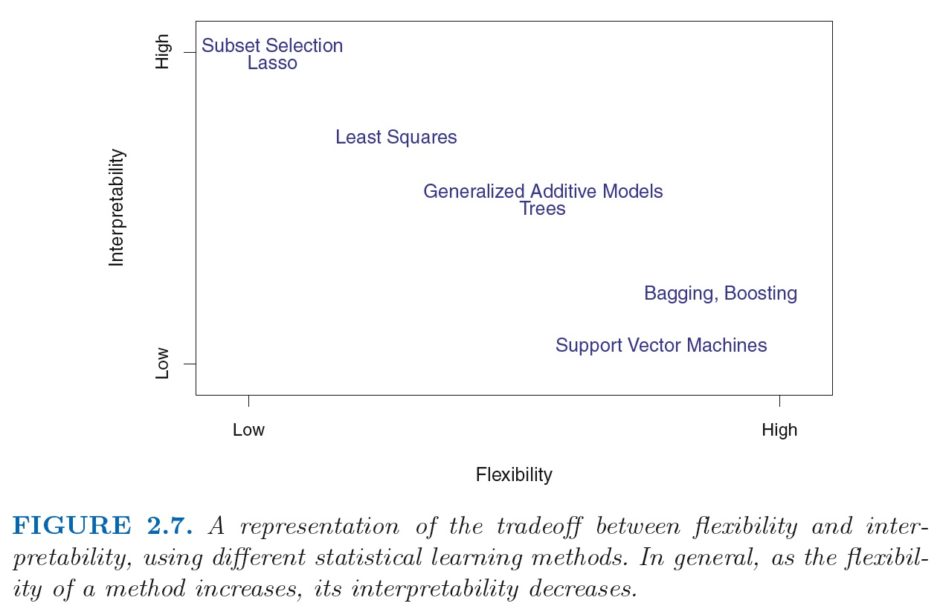
Specifically, what this tradeoff says is this: The more flexible your estimation method gets, the less interpretable it is. OLS, for instance, is relatively inflexible: It imposes a linear relationship between Y and X, which is rather restrictive. But it is also rather easy to interpret, since the coefficient on X is an estimate of the change in Y associated with a one-unit increase in X. And so in the figure above, OLS tends to be low on flexibility, but high on interpretability.
Conversely, really flexible methods–those methods that tend to be very good at accounting for the specific features of the data–tend to be harder to interpret. Think, for instance, of kernel density estimation. You get a nice graph approximating the distribution of the variable you’re interested in, whose smoothness depends on the specific bandwidth you chose, but that’s it: You only get a graph, and there is little in the way of interpretation to be provided beyond “Look at this graph.”
Bonus: Throughout all of the readings I’ve done this week I also came across the following joke (apologies for forgetting where I saw it):
Q: What’s a data scientist?
A: A statistician who lives in San Francisco.