Last week I discussed U-shaped relationships, and how to test for them. This week, I would like to discuss higher-order nonlinear relationship, or relationships that are “more nonlinear” than U-shaped relationships.
There are many ways one can approach the estimation of nonlinear relationships. I will focus only on a handful of them in this post, from least to most nonlinear, and from semiparametric to nonparametric.
A good first step beyond the estimation of a U-shaped relationship would be to estimate the equation
(1) [math]y = \alpha + f(D) + \beta{X} + \epsilon[/math],
where [math]y[/math] is the outcome of interest, [math]D[/math] is your treatment variable, [math]X[/math] is a vector of control variables, and [math]\epsilon[/math] is an error term with mean zero. I assume for the time being that [math]D[/math] is as good as randomly assigned, so that identification is guaranteed.
The difference between equation (1) and the usual linear regression is the term [math]f(D)[/math], where the outcome variable [math]y[/math] is related to the treatment variable [math]D[/math] in a nonlinear fashion by way of the functional form [math]f(\cdot)[/math].
In my own work, one estimator I like to use to model such nonlinear relationships is a restricted cubic spline. Before anything, I should perhaps render unto Caesar the things that are Caesar’s, and note that I learned how to use restricted cubic spline from this set of slides by Maarten Buis, which includes Stata code that you can readily adapt for your own work.
Briefly, when using a restricted cubic spline, you get “a continuous smooth function that is linear before the first knot, a piecewise cubic polynomial between adjacent knots, and linear again after the last knot” (p.1311, Stata Base Reference Manual, Release 13). This is in contrast to a linear spline, which imposes piecewise linear components between the knots; restricted cubic splines should be used in cases where the relationship of interest is “more nonlinear” than what a linear spline allows.
What does a restricted cubic spline look like? Something like this:
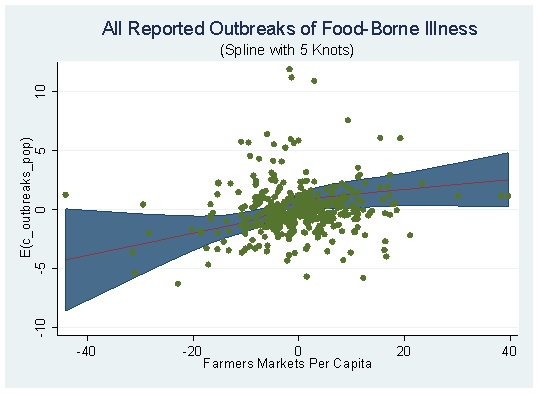
The above figure is from the newest version of my paper on farmers markets and food-borne illness, which I will blog about soon. Because the estimated coefficients from a restricted cubic splines are difficult to interpret by merely looking at them, a picture is literally worth a thousand words when estimating such splines. The above figure, which overlays a scatter plot for [math]y[/math] and [math]D[/math], shows that even when taking into account the nonlinear relationship between those two variables, that relationship looks pretty monotonic (especially considering that there are five knots here, and thus four cubic components between to linear components).
An even cooler thing you can do with the code provided by Buis in his slides is to estimate and plot [math]\frac{\partial{y}}{\partial{D}}[/math], along with its confidence interval, which is the restricted cubic spline analog of the estimated coefficient for [math]D[/math] and its associated confidence interval in the context of a linear regression. For the restricted cubic spline above, the marginal effect looks like this:
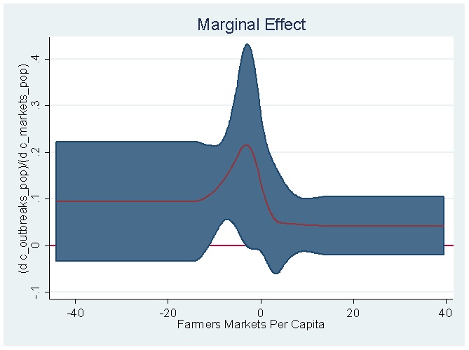
The interpretation of the above figure is as follows: The marginal effect of farmers markets per capita on the number of outbreaks of food-borne illness per capita is everywhere positive, but it is only significant at less than the 5 percent level just a little bit below the mean of the standardized distribution of the treatment variable.
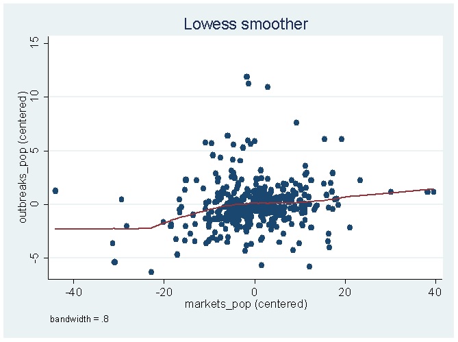
In cases where you want to go full nonlinear, you can use lowess smoothing, which estimates a locally weighted regression of [math]y[/math] on [math]D[/math]. If you are interested in those, the Stata reference manual has a good discussion here. Without any additional options, estimating the relationship in figure 1 by lowess instead of by a restricted cubic spline gives the following:
With that said, I want to reiterate that linear splines, restricted cubic splines, and lowess smoothing are only a handful of a number of potential estimators you can use to estimate nonlinear relationships. If you are interested in reading more on the topic, here is a very partial reading list, in no particular order:
- Henderson and Parmeter (2015), Applied Nonparametric Econometrics.
- Härdle (1992), Applied Nonparametric Regression.
- Pagan and Ullah (1999), Nonparametric Econometrics.
- Yatchew (2003), Semiparametric Regression for the Applied Econometrician.
In closing, I would also like to offer a word of caution. As with any “fancy” procedure (e.g., tobit, Poisson, multinomial logit, etc.) aimed at properly modeling the DGP, there is a danger an inherent danger that once one has learned to use the nonlinear procedures described above, one starts to see everything as a nail. Don’t fall into this trap.
As I have described before, there is an unspoken ontological order in which things are to be tackled in applied econometrics and in most social-scientific applications, it will be much more important to have a reasonable shot at causal identification than it is to accurately model nonlinearities in your data. This means that the procedures described above should be reserved for those cases where you have experimental data, a selection-on-observables design, etc. which yields plausible identification.