Last updated on February 19, 2017
I have mentioned a few times that there is an unspoken ontological order of things in applied work, wherein one first needs to take care of the problem of identification before one should worry about properly modeling the dependent variable’s data-generating process. In other words, before you obsess over whether you should estimate a Poisson or a negative binomial regression, your time is better spend thinking about whether the effect of your variable of interest on your dependent variable is properly identified.
This week, however, I wanted to move away from my usual focus on the identification of causal effects to look at the modeling of DGPs.
Let us take an example from the first article I ever published (and which, to this day, remains my most-cited article). In that article, my coauthor and I were interested in the marketing behavior of the households in our sample. In some time periods, some households happened to be net sellers (i.e., their sales exceeded their purchases), some households happened to be net buyers (i.e., their purchases exceeded their sales), and some households happened to be autarkic (i.e., their neither bought nor sold).
The issue as I saw it was that the same variables (e.g., price, distance from market, etc.) would affect households in different regimes (i.e., the amount of sales of net sellers vs. the amount of purchases of net buyers) in different ways. Moreover, I was interested in the factors that drove households to be either net sellers, autarkic, or net buyers.
After thinking about the decision sequence of the households in our data for a little while, I realized that it could be drawn as follows (with apologies for the lo-fi graph):
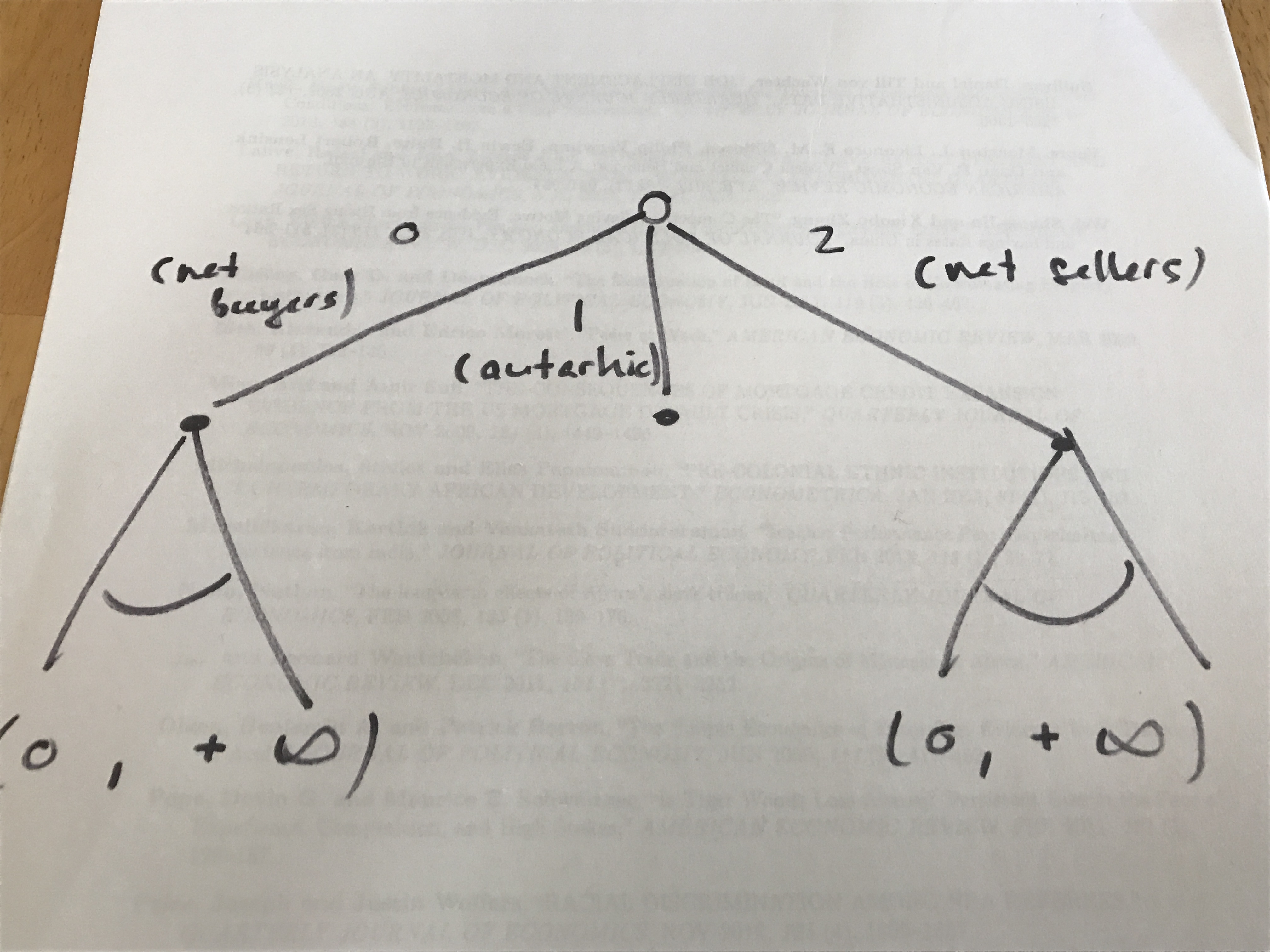
That is, in the first instance, a household decides whether it’ll be net buyer, autarkic, or a net seller. Then, after having chosen whether to be a net buyer, autarkic, or a net seller, the household decides how much it buys (if it has chosen to be a net buyer) or how much it sells (if it has chosen to be a net seller). If it has chosen to remain autarkic, there is no further behavior to study.
Looking at the first stage, note that it is determined by whether a household’s net sales N, which can in theory be any number on the real line, are such that N < 0, N = 0, or N > 0. Because this is an ordered decision when the real line is partitioned in those three regimes, I thought that the first-stage decision lent itself well to an ordered categorical estimator like the ordered probit.
Looking at either side (i.e., net purchases or net sales) of the second stage, it struck me that they were both continuous decision truncated at zero (you can in theory buy or sell any strictly positive amount, but zero is the lower bound on both purchases and sales). Thus, those two decisions lent themselves to some kind of tobit estimator.
I had been thinking a lot about Heckman selection estimators at that time, so one thing that came to mind was that I could write a single likelihood function that would capture the household’s decision problem. The idea was to have three possible participation regimes in the first stage (N < 0, N = 0, or N > 0, or respectively [math] y_{1} \in \{0,1,2\}[/math], and then to have an extent-of-participation decision in cases where [math] y_{1} = 0[/math] or [math] y_{1} = 2[/math]. And obviously, because there was some selection into each of net purchases [math] y_{2}[/math] and net sales [math] y_{3}[/math], there had to be a selection term in each of those extent-of-participation equations.
I was working on all that when I arrived in Madagascar in 2004 to do fieldwork for my dissertation, and I spent many an afternoon writing out likelihood functions in the bar of the Hôtel Colbert in Antananarivo.* Eventually, this is what I ended up with:
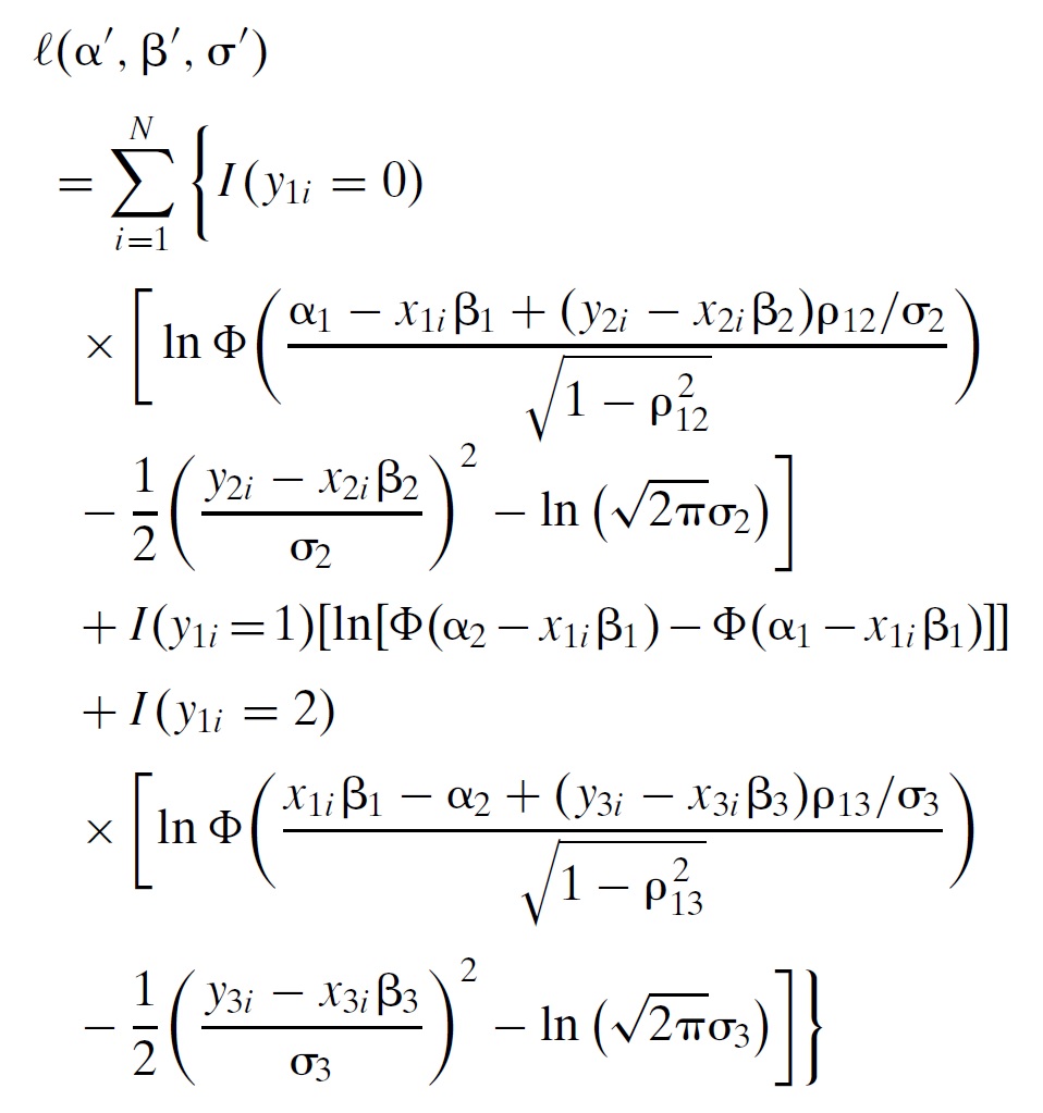
Going through each line after the equality sign:
- The first three lines are the part of the likelihood function that deals with net buyers, both what drives a household into being a net buyer and then how much it purchases conditional on being a net buyer.
- The fourth line is the part of the likelihood function that deals with autarkic households. That is, what drives a household into remaining autarkic, and choosing to neither buy nor sell.
- The last three lines are the part of the likelihood function that deals with net sellers, both what drives a household into being a net seller and then how much it sells conditional on being a net seller.
My coauthor and I called this an “ordered tobit,” and the name seems to have stuck. Since then, a Stata command (oheckman) was developed by Chiburis and Lokshin (2007) to estimate the kind of likelihood function like the one above. Moreover, in a recent article Burke et al. (2015) take the above setup a step further by adding a third stage of selection wherein households first decide whether to be producers or not (specifically, this makes this a “zero-th” stage of selection since that decision occurs before the household decides to be a net buyer, autarkic, or a net seller).
The bottom line is that when faced with complex decisions sequences, it is possible to break those sequences down into different components in order to study what drives each of those components. The way to do this is by combining bits and pieces of likelihood like my coauthor and I did above.
Again, this says nothing about identification, and if you are interested in the causal effect of some variable of interest on complex decision sequences, it is best to be dealing with experimental data so as to not have to worry about identification. But this goes to show that with a little bit of (econometric) structure, it is possible to study more complex decision sequences than what a basic linear projection allows.
* The likelihood function was not the most difficult part of the problem. Given selection issues, the standard errors had to be corrected in a manner similar to Heckman’s original contribution, but accounting for the ordered selection procedure. And then everything needed to be coded by hand using Stata’s “ml” set of commands.