Last updated on October 21, 2018
With panel data, it is not uncommon to present regression results by starting with a pooled ordinary least squares (OLS) regression, then moving on to a specification with fixed effects (FE). If anything, this helps the reader see how important time-invariant unobserved heterogeneity is to your coefficient estimates.
Let y denote your outcome variable, x denote your control variables, and unit denote the unit of observation within which you have variation. If you use Stata, one of the problem that comes from using
xtreg y x, fe i(unit)
instead of
reg y x i.unit
is that none of the R-square measures returned by Stata after the former are in no way comparable to the R-square returned by Stata after the latter. From the “Assessing goodness of fit” section of the xtreg entry in the Stata manual (click on the image to enlarge it):
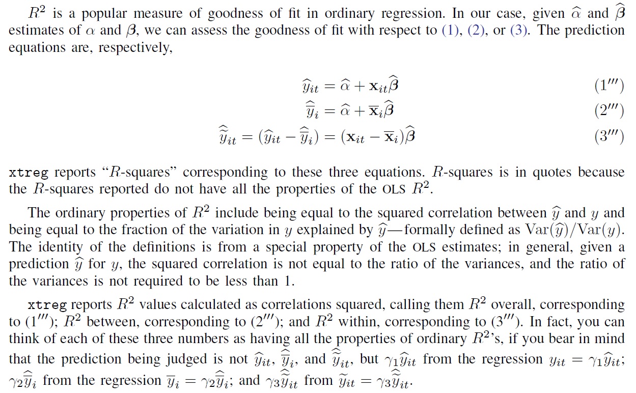
What this means in practice is that if you don’t pay attention to what is going on when making tables of result, you often end up with tables where the R-square in your OLS specification is higher than the R-square in your FE specification. But this is impossible–with the same outcome and control variables, including unit FEs will necessarily raise the R-square since a (usually much) higher percentage of the variation in the outcome is explained by variables on the RHS when using FEs.
This isn’t too bad in and of itself, but of course the first time I noticed this was when someone asked me in a seminar: “Why is your R-square going down instead of up when including fixed effects?,” and I had no good answer other than “I’ll have to check and get back to you on this,” which is seminar-speak for “Beats me.”
Here is a simple (if not terribly elegant) workaround I have come up with and have used and reused in papers where I use the xtreg set of commands. After estimating
xtreg y x, fe i(unit)
I add the following lines of code
egen ybar = mean(y)
gen y2 = (y - ybar)^2
predict resid, e
gen e2 = resid^2
drop resid
egen sse = sum(e2)
egen sst = sum(y2)
gen r2 = 1 - sse/sst
sum r2
drop sse sst y2 e2 ybar r2
The variable r2 is then “right” (i.e., comparable to OLS) R-square.