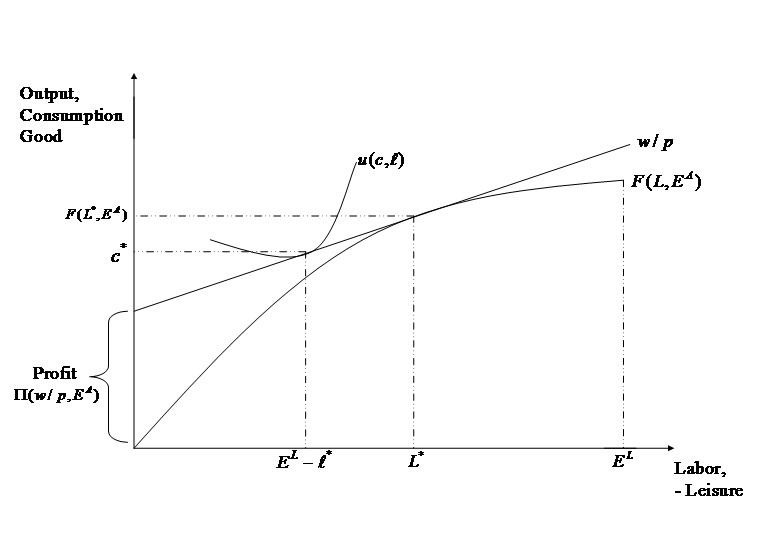
Refer to the figure above, and consider the unitary agricultural model and the case where the Separation Property (Singh et al., 1986) holds, which we discussed in lecture.
The household produces a quantity [math]q=F(L,E^A)[/math] of a staple crop, where [math]L[/math] denotes a household’s labor allocation and [math]E^A[/math] denotes its endowment of land, which we assume fixed in this case. The household consumes a quantity [math]c[/math] of the staple crop. The household also has an endowment of labor time [math]E^L[/math], which it allocates among on-farm labor [math]L[/math], leisure [math]\ell[/math], and market labor [math]L^m[/math], though do note that the household can also hire in labor if it needs to, and that hired labor is denoted [math]L^h[/math]. The household faces wage [math]w[/math] and staple price [math]p[/math].
Pick one of the following three changes in the household’s economic circumstances:
- An increase in the household’s labor endowment, possibly as a result of one of the household’s children attaining adulthood. In other words, the household’s preference structure for consumption and labor remains the same, but the household simply has more labor time,
- An increase in the price of the staple paired with a decrease in the prevailing wage, or
- The adoption of better soil fertility management practices.
Illustrate the change you choose in a graph, and discuss its consequences for the household. Make sure your answer completely describes what happens to the economic circumstances of the household and provides some intuition (or brief explanations) as to why variables change the way they do as a consequence of the change you pick.
I will discuss only the answer to 2 for brevity, but I’d be happy to discuss the answers to 1 and 3 in the comments if there is a demand for them.
Both the increase in [math]p[/math] and the decrease in [math]w[/math] have the same effect, which is to flatten the price line [math]w/p[/math]. The first consequence of this change in prices is that the household’s farm profit increases, given that the price line has a new, higher intercept.
As a result, the household now supplies more of its labor to on-farm production, and so the [math]L^*[/math] increases, which leads to an increase in [math]q = F(L,E^A)[/math] given that the household’s production technology has not changed.
The flattening of the price line also means that the household’s budget constraint flattens as a reflection of the change in relative prices, i.e., leisure is now relatively more expensive than the staple crop, with the obvious result being that the household increases its consumption of the staple crop [math]c[/math].
Whether the household goes from being a net seller of the staple crop initially (since, in the figure above, [math]q>c[/math]) to being autarkic or a net buyer depends on the magnitude of the flattening of the price line; all we know for sure is that the household’s marketable surplus of the crop [math]q-c[/math] decreases.
Likewise, whether the household increases or decreases its consumption of leisure time is not obvious and depends on what is assumed about preferences. That is, it depends on whether, as [math]w/p[/math] decreases and the household attains a higher indifference curve, the tangency between the indifference curve and the price line-cum-budget constraint now happens to the left or to the right of the initial [math]E^L-\ell^*[/math]. This is also key in determining whether the household increases its demand for hired labor [math]L^h[/math].
Indeed, we know the household hires in labor given that (i) its consumption of leisure lies to the left of its allocation of labor on the farm and (ii) that the sum of its on-farm labor allocation and its leisure exceeds its endowment of labor time [math]E^L[/math], and so the household must resort to hiring in labor in order to maximize its utility.
The bottom line is that as the price of the output [math]q[/math] decreases and the the price [math]w[/math] of both the labor input and the household’s leisure increases, the household will face increased incentives to produce on its farm via higher farm profit.
The shift in the household’s budget constraint, which captures the way in which the market trades off the staple crop for leisure increases the incentive to consume the staple crop. Whether the household also consumes more leisure as a consequence of its higher income (because of increased farm profit) will depend on the household’s preferences.
This type of exercise is key in learning two things. First, it teaches students about a new agent — the household — which is both a consumer and a producer, and which most students have never encountered in their prior economics courses.
Second, students learn how crucial market access is to development from this exercise. Indeed, the reason why the household can behave like a profit maximizer and a utility maximizer is because there exist markets for labor and for the staple crop in this example. If either one of those markets were to fail (say, due to high household-specific transaction costs), then the level of welfare the household can attain would be limited by the household’s endowment.
